Estimating the capital cost of modular gas monetization projects

With the ever-increasing demand for energy, the discovery of natural gas resources—especially in the form of unconventional gas such as shale gas, tight gas, coalbed methane (CBM) and gas hydrates—has stimulated a boom in the production of fuels and chemicals.

The total natural gas proven reserves in the U.S. at the end of 2020 was estimated (as wet gas) to be ~473.3 Tft³ (Tcf), according to a recent report published by the U.S. Energy Information Administration (EIA).¹ Furthermore, the EIA estimates that the U.S. has ~2,867 Tft³ of dry natural gas classified as unproved technically recoverable resources.²

Despite an abundance of natural gas resources across the world—an estimated 7,257 Tft³ in proven gas reserves³—more than 30%–40% of these resources remain trapped as what is referred to as ”stranded gas.”^4,5 These resources often remain largely untapped due to the high investment costs associated with their utilization, primarily because they are located in geographically disadvantaged areas.

These stranded gases are often left in the ground, and associated gases produced as a byproduct of crude oil production are either re-injected back into the reservoir or flared—both of which are economically expensive and environmentally disadvantageous.

A recent World Bank report asserted that if all the associated gases that were flared in 2010 had been used for gas-to-liquid (GTL) processing, ~1.5 MMbpd of transportation fuels could have been produced instead of the 320 MMt of unnecessary carbon dioxide (CO₂) emissions it created.⁶ An estimated $20 B was wastefully burned, assuming a price of $4/MMBtu.⁶

Re-injection into ground reservoirs also comes with its fair share of CO₂ emissions, due to the type of compressors used in the process. Market variations and uncertainties in gas prices, low regional demands, inaccessibility to existing pipelines and the remote locations of these unconventional gas reserves (making it economically prohibitive to build new infrastructure) have resulted in these reserves not contributing to the value chain.

Given the financial constraints and difficulty in transporting gas, one solution would be to utilize these resources by transforming them into high-value hydrocarbon liquids, such as gasoline or diesel, that can be easily transported.^7,8 Recently, a significant amount of capital has been invested in large-scale GTL processing plants. Over the years, the technology development domain has also witnessed the emergence of numerous companies that have been developing a small-scale version of these

GTL technologies to provide solutions for stranded/associated gas—especially for processing at much lower volumes—thereby appealing to remote locations with limited economic scope for infrastructure development.

The method of construction of such designs—widening the access to gas processing facilities by building them as movable modular process units that can be easily shipped to and installed at the project location—is referred to as modularization.^9,10,11 These modularized units are considered an efficient solution that enables producers to create the best value and additional revenue from these stranded natural gas resources that would otherwise remain unutilized.

Gas monetization refers to the physical and/or chemical transformation of gas into high value-added products.¹² Of the many available options for gas monetization, GTL is a chemical conversion technology.^13,14 Given the large potential for converting these stranded/associated gases into higher-value fuels and an increase in the number of modular GTL providers, a need has arisen for producers to assess the economic feasibility of installing and operating these modular GTL units at their sites early enough during the initial decision-making phases.

This article seeks to develop an order-of-magnitude correlation to estimate the capital investment required to establish a modular GTL plant for stranded gas monetization. This correlation is intended to help decision-makers and process engineers obtain an order-of-magnitude cost estimate for modular GTL processing units using limited data.

This correlation can be used with any other preliminary cost estimation method prior to developing more detailed techno-economic feasibility reports.

Capital cost estimation methods. The fixed capital investment (FCI) or capital expenditure (CAPEX) of a plant refers to the costs required to design, procure, deliver and install the process equipment, ancillary units, instrumentation, piping, civil and electrical installations, and service facilities required for the process to begin operations.¹⁵

The working capital investment (WCI) is the capital required to cover other expenses until operations can begin. The combined sum of the FCI and the WCI of a processing plant is called the total capital investment (TCI).

Although the level of accuracy may vary based on factors being taken into consideration, some of the commonly used approaches for estimating the TCI of a project include:¹⁵

• Capital cost estimates from the manufacturer
• Capacity ratio with exponent
• Computer-aided tools
• Updates using cost indices such as the Chemical Engineering Plant Cost Index (CEPCI)
• Ratio factors based on equipment cost (Lang factor, Hand factor, etc.)
• Empirical correlations for rough estimates
• Asset turnover ratio/capital ratio.

Companies may also have their own methods of estimation that were developed based on their previous experience with similar projects. The Cost Estimate Classification System, which is recommended by the Association for the Advancement of Cost Engineering (AACE) International, classifies the various phases of project cost estimation for process industries into five different classes. Among these, the estimate that is prepared for the purposes of decision-making at the concept screening level is defined to be the least-detailed estimation class. An estimate that is made at this level of 0%–2% maturity of project definition is designated as Class Level 5 and is often called an order-of-magnitude estimate.

According to the AACE’s classification matrix, the accuracy range of a Class Level 5 provides an order-of-magnitude estimate (OME). The actual price may be as low as 30% less than the OME and as high as 100% greater than the OME (depending on the project type and available information) with the possibility that the ranges can further exceed these limits if additional risks exist.¹⁶

Recently, several order-of-magnitude correlations have been developed for the preliminary assessment of CAPEX during the early stages of decision-making for the cases of gas reforming.^7,8,12,17 This article seeks to develop an order-of-magnitude cost estimation method to enable quick predictions of the FCI required for a proposed modular GTL project.

Data compilation and correlation development. Economic data was collected for existing and proposed modular GTL processes (TABLE 1) from various sources, such as public databases, official company websites, news articles, published techno-economic analyses and status reports like the dedicated mini-GTL technology bulletins published by the World Bank and the Global Gas Flaring Reduction partnership (GGFR). The data available were not always up-to-date and although multiple companies have been reported to be in this business, it was noticed that many of them have stopped pursuing opportunities in this domain due to undisclosed business reasons. It was observed that a few of the successful companies had a merger/partnership with other companies despite originally operating independently. Some of the companies also reported they were now operating under a new name, whereas other technology start-ups became defunct or were not successful in commercialization. Even though attempts were made to contact most of these companies, the authors did not receive a response from some of them. The data presented are those that were compiled from the available sources, while some reflect the information directly obtained from the company.

TABLE 1. Economic data collected for small- to mid-sized GTL processing units. Note: The information provided here is subject to change; the company that developed the technology can provide more accurate and current information on the economics or technology if contacted.^19–28

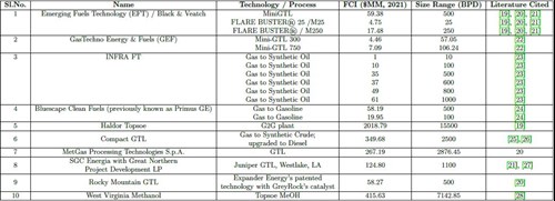TABLE 1. Economic data collected for small- to mid-sized GTL processing units. Note: The information provided here is subject to change; the company that developed the technology can provide more accurate and current information on the economics or technology if contacted.19–28

To update the available data on the required capital investment to that of the year 2021, the authors utilized the CEPCI, based on Eq. 1:

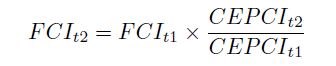                                     (1)

For some providers, the cost data received was limited to the inside battery limit (ISBL), which includes only the major process units and ancillary equipment. Therefore, it was required to calculate the associated capital costs for the outside battery limit (OSBL) expenditure, which includes tank farms, utility systems, etc. This was estimated using Eq. 2:¹²

OSBL expenditure = 0.4 × ISBL expenditure                                          (2)

It was also assumed that the number of production days in a year is a total of 340 days and plant capacities are based on the final product output.

One of the more useful correlations available for the cost function makes use of the processing complexity and capacity ratio with an exponent for the economy-of-scale.¹⁸ The relation used was Eq. 3:¹²

FCI = a°NS^b                                                                                       (3)

where, FCI is the fixed capital investment, a° is an unknown parameter that would be later determined using regression, N is the process complexity in terms of the number of functional units, S is the plant capacity [of the main liquid product(s)] and b is the economy-of-scale exponent with a value less than one, which is also determined through regression analysis of the available data.

Assuming that the various GTL modular plants have a similar number of functional units, the product of the parameters a^o and N is designated as a. Therefore, the modified version of this equation in the context of modular GTL processing units is Eq. 4:

FCI = aS^b                                                                                             (4)

where, FCI is in 2021 $MM and the plant capacity S is in bpd (barrels per day). Due to the variety in the type of products (methanol, ethanol, gasoline, diesel, synthetic oil, etc.) that are obtained from these processes—and since a majority of the available data were presented in terms of bpd—it must be noted that those capacities that were given in metric tpy (tonnes per year) were converted to bpd, considering the appropriate mass, density and conversion factors based on the product.

To ascertain the unknown parameters a and b, the equation was written as Eq 5, taking logarithms on both sides:

log(FCI) = b log(S) + log(a)                                                                    (5)

A log-log plot shown in FIG. 1 was generated using the compilation of data listed in TABLE 1. The values of a and b were found to be 0.12 and 0.96, respectively, by fitting a linear regression model to the log-log data.

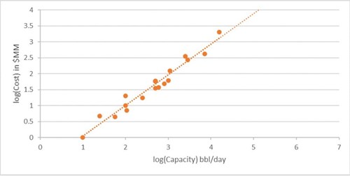FIG. 1. A log-log plot of FCI vs. capacity S.

TABLE 1. Economic data collected for small- to mid-sized GTL processing units. Note: The information provided here is subject to change; the company that developed the technology can provide more accurate and current information on the economics or technology if contacted.^19–28

The final empirical correlation can be written as Eq. 6:

FCI = 0.12(S)^0.96                                                                             (6)

The equation is valid for the capacity range from 10 bpd–15,500 bpd. The percentage error between the original FCI and the FCI calculated using Eq. 6 was found to be no more than ± 2%−50% for each entry listed in TABLE 1, indicating the prediction is indeed within the approved limits for AACE Class Level 5.

Using the correlation. To illustrate the use of the correlation, the following case is examined. Assume a GTL plant that will have a 1,100-bpd capacity. Using Eq. 6, Eq. 7 is calculated as:

FCI = 0.12(1,100)^0.96 = $99.75 MM                                                    (7)

The 2021-updated FCI value reported for the Juniper GTL plant in West Lake, Louisiana (U.S.) is $124.80 MM. Although the FCI value predicted by the proposed correlation is 20% less than the reported FCI for a plant of similar size, the error is within the acceptable range for Class Level 5 order-of-magnitude estimates as described above.

Takeaways. The correlation proposed in Eq. 6 may be used as one of the order-of-magnitude estimates for a small-scale GTL project during its preliminary design phases. The prediction accuracy obtained with the equation is consistent with the requirements for a AACE Class Level 5 cost estimate and, therefore, can be used for engineering calculations in the conceptual design phases. However, it is recommended that it be used with some level of caution, just as other methods that exist for obtaining similar cost estimates. GP

 

LITERATURE CITED

1. Energy Information Administration (EIA), “U.S. crude oil and natural gas proved reserves, year-end 2021,” December 2022, online: https://www.eia.gov/naturalgas/crudeoilreserves/
2. U.S. Energy Information Administration (EIA), “Natural gas explained: How much natural gas is left,” online: https://www.eia.gov/energyexplained/natural-gas/how-much-gas-is-left.php
3. U.S. Energy Information Administration (EIA), “Frequently asked questions (FAQs),” online: https://www.eia.gov/tools/faqs/faq.php
4. Khalilpour, R. and I. Karimi, “Evaluation of utilization alternatives for stranded natural gas,” Energy, Vol. 40, No. 1, 2012.
5. Thackeray, F. and G. Leckie, “Stranded gas: A vital resource,” Petroleum Economist, Vol. 69, No. 5, 2002.
6. Fleisch, T., “Associated gas utilization via mini(GTL),” World Bank, Open Knowledge Repository, online: https://openknowledge.worldbank.org/handle/10986/21976
7. Alsuhaibani, A. S., S. Afzal, N. O. Elbashir and M. M. El-Halwagi, “An evaluation of shale gas reforming technologies—Part 1: Technology overview and selection,” Gas Processing & LNG, August 2022.
8. Alsuhaibani, A. S., S. Afzal, N. O. Elbashir and M. M. El-Halwagi, “An evaluation of shale gas reforming technologies—Part 2: Cost and carbon intensity estimation,” Gas Processing & LNG, October 2022.
9. R. C. Allen, R. C., D. Allaire and M. M. El-Halwagi, “Capacity planning for modular and transportable infrastructure for shale gas production and processing,” Industrial & Engineering Chemistry Research, Vol. 58, No. 15, December 2018.
10. Al-Fadhli, F. M., H. Baaqeel and M. M. El-Halwagi, “Modular design of carbon-hydrogenoxygen symbiosis networks over a time horizon with limited natural resources,” Chemical Engineering and Processing, Vol. 141, 2019.
11. Barron, A., N. Chrisandina, A. L´opez-Molina, D. Sengupta, C. Shi and M. M. El-Halwagi, “Assessment of modular biorefineries with economic, environmental, and safety considerations,” Chapter 9, Biofuels and Biorefining, Elsevier, 2022.
12. Zhang, C. and M. M. El-Halwagi, “Estimate the capital cost of shale-gas monetization projects,” Chemical Engineering Progress, Vol. 113, No. 12, 2017.
13. Gabriel, K. J., M. Noureldin, M. M. El-Halwagi, P. Linke, A. Jiménez-Gutiérrez and D. Y. Martínez, “Gas-to-liquid (GTL) technology: Targets for process design and water-energy nexus,” Current Opinion in Chemical Engineering, Vol. 5, Elsevier, August 2014.
14. Bao, B., M. M. El-Halwagi and N. O. Elbashir, “Simulation, integration, and economic analysis of gas-to-liquid processes,” Fuel Processing Technology, Vol. 91, No. 7, 2010.
15. El-Halwagi, M. M., Sustainable design through process integration: Fundamentals and applications to industrial pollution prevention, resource conservation, and profitability enhancement, 2nd Ed., IChemE/Elsevier, 2017.
16. American Association of Cost Engineering (AACE), “International recommended practice no. 56r-08: Cost estimate classification system—as applied in engineering, procurement, and construction for the building and general construction industries,” 2019.
17. Lόpez-Molina, A., D. Sengupta, C. Shi, E. Aldamigh, M. Alandejani and M. M. El-Halwagi, “An integrated approach to the design of centralized and decentralized biorefineries with environmental, safety, and economic objectives,” Processes, Vol. 8, No. 12, 2020.
18. Tsagkari, M., J.-L. Couturier, A. Kokossis and J.-L. Dubois, “Early-stage capital cost estimation of biorefinery processes: A comparative study of heuristic techniques,” ChemSusChem, Vol. 9, No. 17, 2016.
19. “MiniGTL Technology Bulletin Volume 7,” September 2020, online: https://pubdocs.worldbank.org/en/829751598037226396/Mini-GTL-Bulletin-No-7-September-2020.pdf
20. “MiniGTL Technology Bulletin Volume 6,” July 2019, online: http://rockymountaingtl.com/wp-content/uploads/2019/11/Mini-GTL-Bulletin-No-6 July-2019.pdf
21. “Global Gas Flaring Reduction (GGFR) technology overview—Utilization of small-scale associated gas,” September 2020, online: https://pubdocs.worldbank.org/en/662151598037050211/GGFR-Small-scale-gas-utilization-technology-Summaries-September-2020.pdf
22. Gas Technologies LLC, Private communication, December 2020.
23. “INFRA GTL Investment Calculator*,” February 2020, online: https://en.infratechnology.com/calculator/
24. Bluescape Clean Fuels, Private communication, December 2020.
25. “Compact GTL presentation,” September 2020, online: http://www.compactgtl.com/wp-content/uploads/2015/04/CompactGTL-presentation-for-IGTC-2015-English-version.pdf
26. “Compact GTL,” September 2020, online: https://www.compactgtl.com/about/projects/
27. “Juniper GTL to invest $100M to retrofit plant to new small-scale GTL facility in Louisiana,” Green Car Congress, September 2013, online: https://www.greencarcongress.com/2013/09/20130907-juniper.html
28. “Gov. Justice announces West Virginia Methanol Inc. to build $350 million methanol plant, bring high-paying jobs to Pleasants County,” October 2020, online: https://governor.wv.gov/News/press-releases/2020/Pages/Gov.-Justice-announces-West-Virginia-Methanol-Inc.-to-build-%24350-million-methanol-plant,-in-Pleasants-County.aspx

 

 

 

Ashwini Ravindran is a PhD student at the Wm Michael Barnes '64 Department of Industrial and Systems Engineering, Texas A&M University. She earned a BTech degree in chemical engineering from the National Institute of Technology Calicut, India and an MEng degree in chemical engineering from Texas A&M University, College Station, Texas (U.S.). Her research activities are in process integration, optimization and network-based data mining.

 

Mahmoud M. El-Halwagi is a Professor and holder of the Bryan Research and Engineering Chair and the Managing Director of the Gas and Fuels Research Center at Texas A&M University, College Station, Texas (U.S.). Dr. El-Halwagi’s main areas of expertise are sustainability, process integration, synthesis, design, operation and optimization. He is the author of three textbooks, the co-author of more than 500 referenced papers and book chapters, and the co-editor of 10 books. Dr. El-Halwagi is the recipient of several awards, including the AIChE Computing in Chemical Engineering Award and the AIChE Sustainable Engineering Forum Research Excellence Award. He earned his BS and MS degrees from Cairo University and his PhD from the University of California, Los Angeles.

Related Articles