
Optimization of BOG management during LNG unloading with dynamic simulation
In LNG receiving terminals, the dynamic nature of boiloff gas (BOG) generation in the unloading process can be difficult to understand, and BOG management can be challenging. Dynamic simulation has been used in a few limited studies in this field, but a systematic approach is lacking for conducting simulations, data collection and analysis.
In this study, dynamic simulation, experiments and analysis are used to model the entire LNG unloading process, to collect and analyze experimental data, to gain insights into system behavior and to optimize the unloading process. This optimization is performed with respect to two important decision variables—the recirculation flowrate and the bypass flowrate—to reduce operating cost.
By using designed experiments and analysis as powerful tools, the dynamic simulation and data collection/analysis can be carried out more efficiently and more accurately. Insights are gained regarding BOG generation behavior during the unloading process that can be used to guide operations, and cost savings goals are achieved through process optimization.
Process background and previous research. Since LNG is stored and transported at an approximate temperature of –160°C, there will be continuous heat leakage into LNG storage tanks and pipelines. Mechanical equipment, including low-pressure (LP) and high-pressure (HP) pumps, will also send heat into the LNG stream. These factors (together with other effects, like tank volume displacement under unloading operations and flashing due to pressure difference) result in the generation of BOG in the system. Managing BOG in LNG terminals is challenging since it involves safety, hydraulics, turndown, transient behavior, economics, and process and equipment selection for BOG handling.
Processes vary from terminal to terminal. A typical LNG receiving terminal comprises an unloading facility (i.e., jetties, unloading arms and associated pipelines, etc.), storage tanks, a BOG handling facility (i.e., compressors, recondensers, etc.), and an LNG regasification facility (i.e., pumps, vaporizers, etc.). A simplified LNG receiving terminal process flow diagram is shown in Fig. 1.
Previous research1–6 has used numerical modeling or equations of state to study the internal behavior of BOG generation inside LNG storage tanks. Some researchers7 have proposed optimal operating conditions for an LNG regasification facility. Others8 studied and improved BOG recondensation operations in an LNG receiving terminal. A method for optimizing BOG compressor operations has also been proposed.9 Studies of LNG receiving terminals have focused on system performance optimization to reduce costs10–13 and make operations smoother.14
However, a systematic approach is missing regarding the data collection and analysis used for a dynamic system like an LNG receiving terminal, which is affected by multiple variables. Dynamic simulation has been used in only a few limited studies due to its challenging nature, and the method for conducting the simulation lacks efficiency in terms of data collection and analysis. In this article, dynamic simulation is used, along with designed experiments and statistical analysis, to study the unloading process of LNG receiving terminals, to optimize unloading operations and to achieve cost savings.
LNG unloading operations. In Fig. 1, valve V3 (typically 24 in.–32 in.) is the unloading valve, and the much smaller-sized V4 valve (typically 2 in.) is the bypass valve. When no ship unloading operation is taking place, V3 is closed while recirculation valves V1 and V2 are open, and part of the LNG flow from the low-pressure (LP) pumps is sent through the recirculation line into the unloading pipeline to keep the unloading system cold (at –160°C to –150°C).
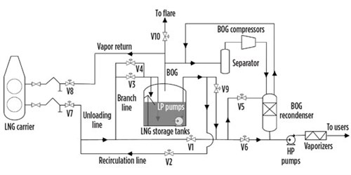 |
| Fig. 1. A simplified LNG receiving terminal process flow diagram. |
Most of the recirculation flow is sent downstream via V1, while a small portion is returned to the tank via bypass valve V4 to keep the branch pipeline cold. The recirculation flowrate is controlled such that the recirculation outlet and inlet temperatures have a recommended difference of approximately 3°C–5°C.13 By increasing the recirculation flowrate, the temperature difference will decrease, and vice versa. The recirculation flow pressure is kept relatively high (around 1,000 KPa) to prevent LNG from vaporizing and to accommodate the downstream (recondenser) operating pressure. This process is called recirculation.
To prepare for unloading an LNG carrier, the unloading pipeline is depressurized since the recirculation system pressure is much higher than the carrier tank pressure, which is slightly above atmospheric pressure. This is achieved by closing recirculation valves V1 and V2 while keeping open bypass valve V4. A closed-loop system with only one exit to the LNG storage tank is formed, and the pressure is gradually released to the tank. This process is called depressurization.
Other things to prepare for unloading after ship berthing include ship-side and shore-side communication, and unloading arm connection and purging, which will typically take a few hours before unloading can start. The bypass valve V4 is then closed. The valves in the unloading pipeline (V3 and V7) and the valves on the ship side are open. Once the unloading path is clear and both sides are ready, the ship unloading can formally begin. The maximum unloading rate reaches approximately 12,000 m3/hr.
Dynamic simulation. In LNG receiving terminals, the entire BOG system is in dynamic operational mode and never achieves a steady state; therefore, dynamic simulation is the correct way to analyze the system. As explained in the unloading operations section, one unloading cycle is made up of recirculation, depressurization and ship unloading processes. After ship unloading is finished, the system returns to the recirculation stage and a new cycle begins.
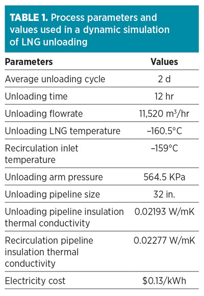
A dynamic simulation model for the unloading process, as shown in Fig. 2, is built using a proprietary process simulator with a Peng-Robinson-Stryjek-Vera equation of state (PRSV EOS) fluid package. Using this model, the entire unloading process can be modeled by switching the valves. The process parameters and values are incorporated into the dynamic model or used for cost calculations, as shown in Table 1.
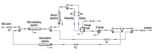 |
| Fig. 2. Dynamic simulation model for LNG receiving terminal unloading process. |
 |
Experiments and analysis. The unloading process can be analyzed using structured sets of experiments, or designed experiments, that allow for efficient collection and analysis of data.
For the unloading process, the decision variables are the recirculation flowrate Qr and the bypass flowrate Qb, since they determine the pipeline temperature and, therefore, the amount of BOG produced. The constraint for the recirculation flowrate is that the recirculation inlet and outlet temperature difference is within 3°C–5°C. The bypass flowrate is in the range of 1 m3/hr–10 m3/hr, based on experience.
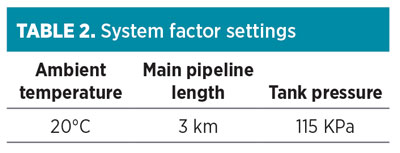
The main physical system factors include the ambient temperature, the length of the main unloading pipeline and the storage tank operating pressure. The full experimental design can be used to test how these factors affect the system performance and how they interact with one other. However, only one combination is taken to illustrate the methodology and to study the unloading process. The optimal recirculation flowrate and the bypass flowrate can be determined based on system performance measures (i.e., the experiment responses): the amount of BOG generated by the process, the pump cost (PC), the compressor cost (CC) and the total cost (TC). The objective is to minimize the total cost. The system factor settings are shown in Table 2.
 |
By running the dynamic simulation model, using the previously outlined system factor settings, the valid range for Qr is 120 m3/hr–220 m3/hr, based on achieving the recirculation inlet and outlet temperature difference of 3°C–5°C.
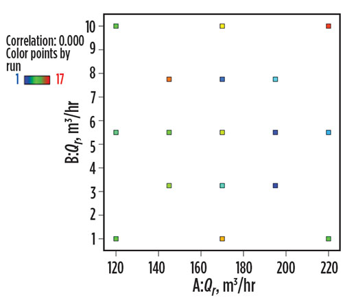
Although standard designs are available, like Central Composite Design (CCD) and D-optimal designs, they are not sufficiently flexible to model the required design space. The experimental designs used in this study are specifically customized as shown in Fig. 3.
 |
|
Fig. 3. Customized experimental design for LNG unloading study. |
After running the simulations with the designed experiments, the experiment analysis can be done using a commercial design software package. Based on the inherent features of the system to be studied, the resulted response surface model can be linear, quadratic, cubic or even higher-order models. The analysis of variance (ANOVA) can be performed, and the significance of the model can be checked. The model graphs, including main and interaction effects, contour plots and 3D surface plots (if applicable) can be obtained. The optimization can then be conducted based on the factor constraints and the system objective.
Operating power consumption cost analysis. Since only the unloading process is studied here, the power consumption of the LP pump is considered only at the recirculation stage of the specific recirculation flowrate used for cooling. During the depressurization and ship unloading stages, the LP pump may still be sending fluids downstream, but none are related to the unloading process; therefore, the LP pump’s power consumption is not considered. The BOG compressor, however, is working constantly to handle the BOG generated during the unloading process.
The pump power consumption from the unloading process can be calculated with Eq. 1:15
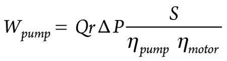 |
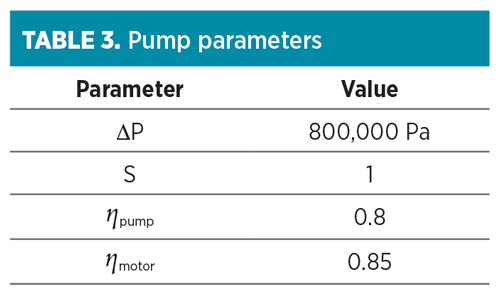 |
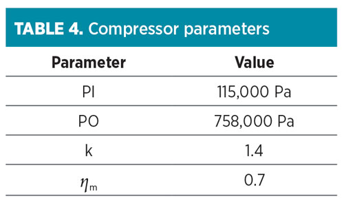
The pump parameters are presented in Table 3. The compressor power consumption cost can be calculated with Eq. 2:11
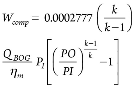 |
The compressor parameters are presented in Table 4.
 |
Optimization procedure. After the dynamic simulation model is built, and the experimental design and the constraints or boundary conditions are set, a procedure can be used to find the optimal solution.
The combinations of the experiments should first be run. For each combination, the entire process should be run—i.e., recirculation and depressurization to ship unloading—and the BOG generated from the corresponding unloading process at each stage should be recorded. The three stages of the unloading process are simulated in order, and the ending conditions of the previous stage are used as the starting point of the next stage. After each combination is run, the total amount of BOG generated should be recorded, together with the Qr used, which can be used for calculating the PP, CC and TC.
After all combinations are run, an analysis can be carried out to find the relationship between the decision variables (Qr and Qb) and the system performance (the amount of BOG generated and the costs incurred). Based on these data, an optimization can be performed to determine the optimal factor settings for minimizing the total cost.
Study results. The model of the BOG generation in terms of Qr and Qb is linear. ANOVA analysis shows that the model is significant, and the diagnostics look favorable. This analysis can be used for analyzing and predicting the system performance. Fig. 4 shows the normal probability plot of residuals, and Fig. 5 shows the residuals vs. predicted plot.
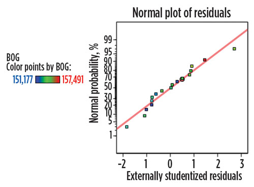 |
| Fig. 4. Normal probability plot of residuals. |
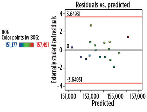 |
| Fig. 5. Residuals vs. predicted plot. |
The BOG main effects plot (Fig. 6) and the contour plot (Fig. 7) show that when Qr increases, the amount of BOG generated decreases. Bypass flowrate Qb is exactly the opposite. When Qb increases, the amount of BOG generated also increases. This observation is reasonable because when Qr increases, the pipeline temperature decreases, meaning that a smaller amount of LNG vaporizes into BOG. Bypass flow Qb goes directly into the storage tank, so when Qb increases, more BOG is generated due to heat input from environment, pressure drop flashing and volume displacement.
 |
| Fig. 6. BOG main effects plot. |
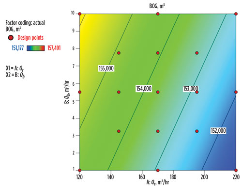 |
| Fig. 7. BOG contour plot. |
Most of the BOG is generated in the ship unloading stage, compared to the recirculation and depressurization stages. When ship unloading starts, a sharp jump is seen in BOG inflow sent to the tank. The BOG inflow decreases and stabilizes in approximately 30 min for the 3-km main pipeline. Fig. 8 (copied from the dynamic simulation strip chart) shows typical BOG generation at the beginning of the ship unloading stage. After recirculation is stopped and during the depressurization stage, the heat input to the pipeline causes vapor formation, and the depressurization process itself causes LNG flashing into BOG. When unloading starts, the LNG from the carrier pushes the vapor in the unloading pipeline into the tank, which causes a sharp increase in BOG generation.
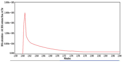 |
| Fig. 8. BOG generation at the beginning of LNG ship unloading. |
Due to the large unloading flowrate and the cold temperature of the LNG from the carrier, the unloading pipeline is quickly cooled, and the BOG generation decreases and stabilizes at a level correlating with the volume displacement of LNG into the tank. Therefore, tank pressure should be closely monitored at the beginning of ship unloading, especially in the first hour or so.
The rate of BOG generation during the recirculation stage is constantly rising (see solid red line in Fig. 9), which is shown in the dynamic simulation strip chart. Investigation shows that this is due to the temperature rise and, therefore, the vapor fraction increase in the branch pipeline. The recirculation and main unloading pipeline temperatures (shown as the red dotted line in Fig. 9) are relatively stable because of the larger recirculation flowrate compared to the bypass flowrate. Since the bypass flowrate is low, the constant heat input from the environment causes the branch pipeline temperature (the dot-dash blue line in Fig. 9) and the vapor fraction (the dashed black line in Fig. 9) to rise constantly.
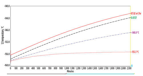 |
| Fig. 9. BOG generation during the recirculation stage. |
Moreover, the recirculation system pressure is high, and a large pressure drop is seen through bypass valve V4 to reduce the pressure to the same level as the tank pressure, which is slightly above atmospheric pressure. The large pressure drop causes more LNG to flash into BOG. The BOG generated at the depressurization stage is low and negligible due to the short time span and the limited holding volume inside the pipeline.
The PC of power consumption is directly proportional to Qr, which can be seen from Eq. 1. Since Qb is a portion of Qr, it does not affect PC directly. Fig. 10 shows the PC main effect plot.
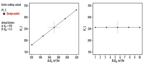 |
| Fig. 10. Pump cost main effect plot. |
The CC of power consumption is directly proportional to the amount of BOG generated. When Qr increases, CC decreases; when Qb increases, CC also increases. This correlation is reasonable since it explains how BOG generation is related to Qr and Qb. Fig. 11 illustrates the CC main effect plot.
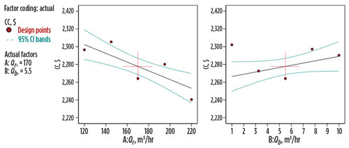 |
| Fig. 11. Compressor cost main effect plot. |
From this analysis, when Qr increases the pump cost also increases, while the compressor cost decreases. Therefore, Qr creates a trade-off between the pump operating cost and the compressor operating cost.
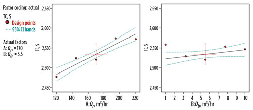
The TC fits into a linear model with Qr and Qb. When Qr increases, total cost goes up; this is also true for Qb. Fig. 12 shows the TC main effect plot.
 |
| Fig. 12. Total cost main effect plot. |
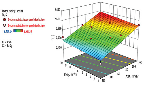
Optimization can be carried out based on the response surface model that is obtained to find the optimal solution to minimize the TC. The results show that the lowest TC occurs when both Qr and Qb are at the lowest levels—120 m3/hr and 1 m3/hr, respectively. This recirculation flowrate corresponds to the recirculation inlet and outlet temperature difference of 5°C. Fig. 13 illustrates the 3D surface plot of TC. By simply switching from a 3°C difference to a 5°C difference, the annual cost savings is approximately 5%.
 |
| Fig. 13. Three-dimensional surface plot of the total cost. |
This result is based on the LP pump and BOG compressor operating costs only and is applicable to LNG receiving terminals that do not have a high-pressure (HP) BOG compressor installed. If an HP BOG compressor exists, its cost should also be included in the calculation. In that case, the recondensation process must be taken into consideration, as it is related to the intensity of operation of the HP BOG compressor—i.e., the amount of BOG that cannot be condensed by the recondenser due to a limited amount of LNG sendout or another reason.
Recommendations. BOG management in LNG receiving terminals is challenging. This article proposes a powerful and efficient way of performing a dynamic simulation and collecting and analyzing data, using designed experiments and statistical analysis. The LNG receiving terminal unloading process has been studied using this methodology. Insights have been gained on BOG generation behavior during the unloading process that can be used to guide operations. Process optimization has been carried out to adjust the recirculation and bypass flowrates to achieve cost savings.
The results show that it is favorable to set both flowrates at the lowest settings allowed by the system. Simply switching from high-level flow settings to low-level flow settings can give an approximate cost savings of 5%/yr. However, this study is based on LNG terminals that have no HP BOG compressor installed. If an HP compressor is installed, then its cost must be included and the recondensation process must be studied again. GP
Nomenclature
Q Flowrate, m3/hr
P Pressure, Pa
η Efficiency
S Safety factor
W Power, W
∆P Pressure drop, Pa
k Specific heat ratio
r Recirculation
b Branch
m Mechanical
comp Compressor
I Inlet
O Outlet
Literature cited
1 Roh, S., G. Son, G. Song and J. Bae, “Numerical study of transient natural convection in a pressurized LNG storage tank,” Applied Thermal Engineering, Vol. 5, 2013.
2 Heestand, J., C. W. Shipman and J. W. Meader, “A predictive model for rollover in stratified LNG tanks,” AIChE Journal, Vol. 29, 1983.
3 Chan, S. T., “Numerical simulation of LNG vapor dispersion from a fenced storage area,” Journal of Hazardous Materials, Vol. 30, 1992.
4 Bates, S. and D. S. Morrison, “Modeling the behavior of stratified liquid natural gas in storage tanks: A study of the rollover phenomenon,” International Journal of Heat Mass Transfer, Vol. 40, 1997.
5 Dimopoulos, G. G. and C. A. Frangopoulos, “A dynamic model for liquefied natural gas evaporation during marine transportation,” International Journal of Thermodynamics, Vol. 11, No. 3, 2008.
6 Adom, E., S. Z. Islam and X. Ji, “Modelling of boil-off gas in LNG tanks: A case study,” International Journal of Engineering and Technology, Vol. 2, Iss. 4, 2010.
7 Huang, S., D. Coyle, J. Cho and C. Durr, “Select the optimum extraction method for LNG regasification,” Hydrocarbon Processing, Vol. 83, 2004.
8 Kim, D., Y. Ha, I. Park and Y. Yoon, “Study on the improvement of BOG recondensation process at LNG receiving terminal,” KIKAS, Vol. 5, 2001.
9 Shin, M. W., D. Shin, S. H. Choi, E. S. Yoon and C. Han, “Optimization of the operation of boiloff gas compressors at a liquefied natural gas gasification plant,” Industrial and Engineering Chemistry Research, Vol. 46, 2007.
10 Lee, C. J., Y. Lim and C. Han, “Operational strategy to minimize operating costs in liquefied natural gas receiving terminal using dynamic simulation,” Korean J. Chem. Eng., Vol. 29, Iss. 4, 2012.
11 Wu, M., Z. Zhu, D. Sun, J. He, K. Tang, B. Hu and S. Tian, “Optimization model and application for the recondensation process of boil off gas in a liquefied natural gas receiving terminal,” Applied Thermal Engineering, Vol. 147, 2019.
12 Park, C., C. J. Lee, Y. Lim, S. Lee and C. Han, “Optimization of recirculation operating in liquefied natural gas receiving terminal,” Journal of Taiwan Institute of Chemical Engineers, Vol. 41, 2010.
13 Lee, C. J., Y. Lim and C. Han, “Operational strategy to minimize operating costs in liquefied natural gas receiving terminal using dynamic simulation,” Korean J. Chem. Eng., Vol. 29, Iss. 4, 2012.
14 Li, Y. J. and Y. Li, “Dynamic optimization of boil-off Gas (BOG) fluctuations at and LNG receiving terminal,” Journal of Natural Gas Science and Engineering, Vol. 30, 2016.
15 Seider, W. D., J. D. Seader and D. R. Lewin, Product and Process Design Principles: Synthesis, Analysis, and Evaluation, John Wiley & Sons, Hoboken, New Jersey, 2004.
 |
Scott Su is a Senior Process Engineer with ProPEng Inc. in Calgary, Alberta, Canada. He received a BSc degree in chemical equipment and mechanical engineering from Liaoning University of Petroleum and Chemical Technology in 1995, and an MSc degree in mechanical engineering from the University of Calgary in Alberta, Canada. Mr. Su is a registered professional engineer in Alberta (Canada) and in Texas and Pennsylvania (U.S.).


Comments